CS180 Project NeRF

Part 1: Neural Fields

The hidden layers are set at 256. I followed the spec for the overall model architecture.

For changing hyperparameters of the neural network, here’s what I tried:

changing hidden layer size to 1024

changing highest frequency level of sinusodial positional encoding to 20.

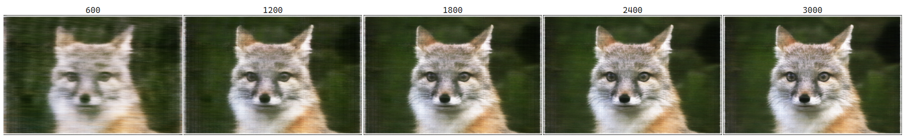
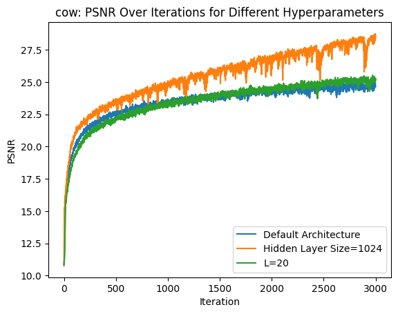
Here are the PSNR curves for the fox image:

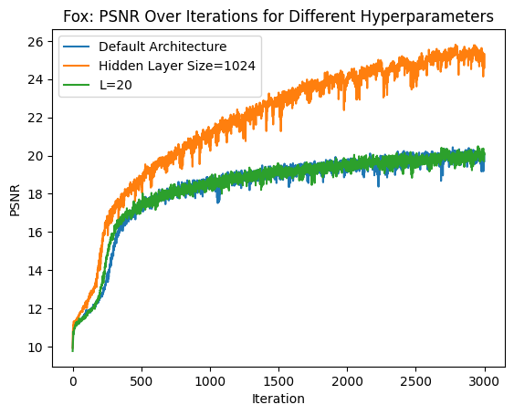
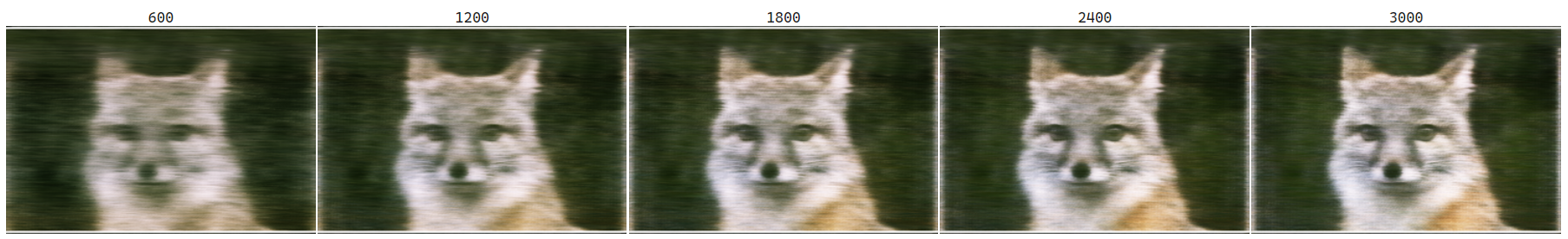
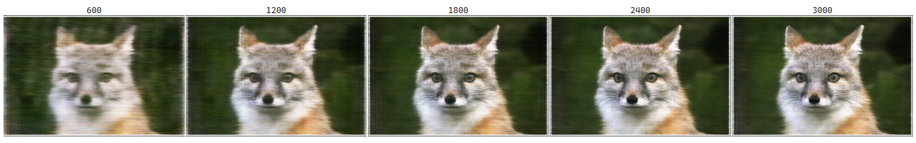
Overall, increasing the size of the model led to better results, while increasing the highest frequency level didn’t have much of an impact. And the network’s predictions across training iterations:

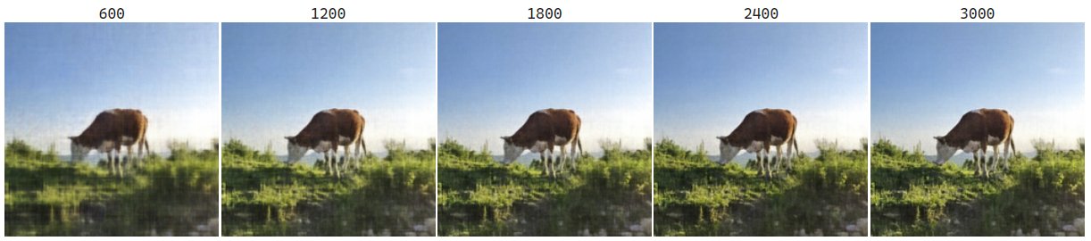
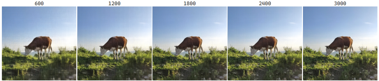
I also tried the same experiments on my own image. PSNR loss curve:

Prediction results:

Part 2: Neural Radience Field

General Approach

Create Rays from Cameras

For camera to world coordinates, I wrote functions transform according to the spec and helper pad_coords_to_homogeneous to pad the 2D coordinates with a homogenous third dimension.

For pixel to camera coordinates, I calculated the K intrinsic matrix:

{K} = \begin{bmatrix}f_x & 0 & o_x \\0 & f_y & o_y \\0 & 0 & 1\end{bmatrix}

To get the camera coordinates from pixel coordinates, I did

{K}^{-1} s \begin{bmatrix}u \\v \\1\end{bmatrix}=\begin{bmatrix}x_c \\y_c \\z_c\end{bmatrix}

To calculate the ray origin and ray directions, I used $R^{-1}_{3x3}$ and $t$ from the camera-to-world matrix. Before finding ray directions, I converted the pixel coordinates to camera coordinates, and they the camera coordinates to world coordinates.

Sampling

I took the second approach and sampled across all images gloablly to get N rays from all images. To sample points, I added the option to include tiny perturbations to the uniformly separated points along the ray. The sampling is encapsulated within the NeRFSampler for later training and reuse.

Model Architecture

I followed the architecture on the spec to create the NeRF model. The hidden layers have size 256. For the layers following skip connections, the input dimensions are expanded to account for the concatenation. For positional encodings, the PE for coordinate has L=10, and the PR for ray directions has L=4.

Volume Rendering

Following in the hints on the spec, I used torch.cumsum to calculate the $T_i$ array. To account for the $i-1$ term on the summation, I padded the densities with 0 in front. The rest of the procedure follows the equation. Unfortunately, I had a hard time vectorizng calculations across rays, so the volume rendering happens one ray at a time. A future improvement could be to vectorize everything to speed up calculations.

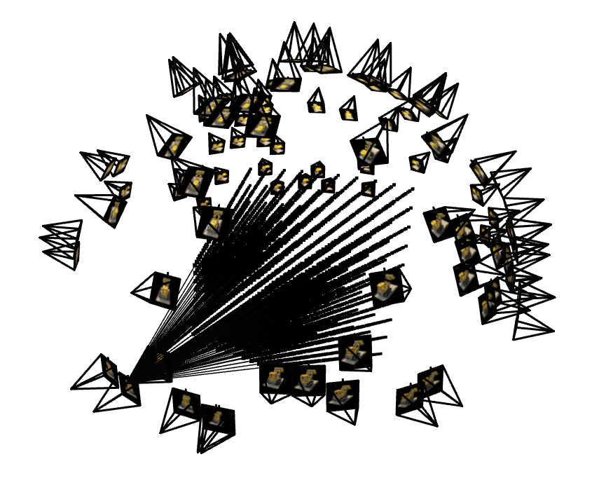
Visualization of Sampled Rays

This is the visualization of sampling at an iteration (with less rays shown to prevent cluttering):

Just to make sure that the sampling worked, I also tried a snippet to sample uniformly across one image. NOTE that this is just for checking code, the actual training used sampling strategy shown above.

Training Process

For training, I set the following hyperparamters:

adam learning rate: 1e-3.

gradient steps: 3600

batch size (number of rays for each gradient step): 1024

number of samples along each ray: 64

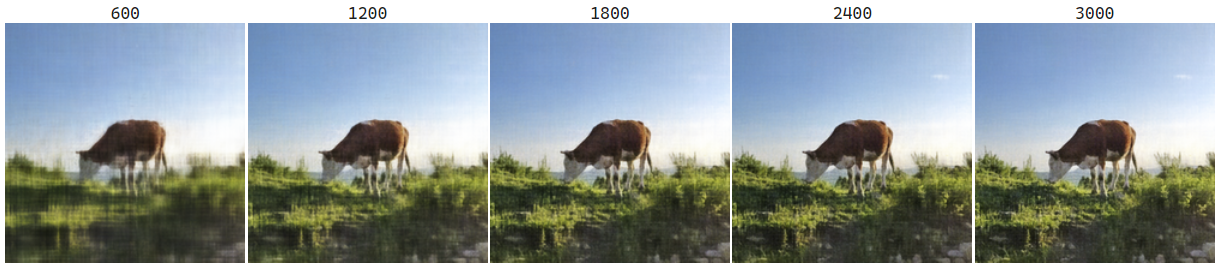
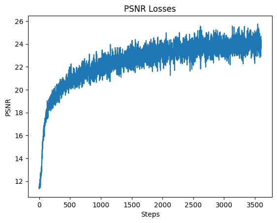
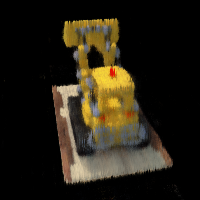
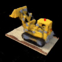
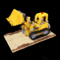
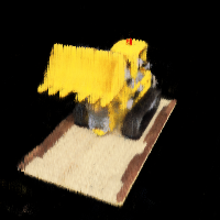
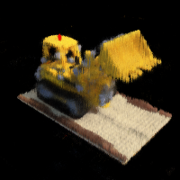
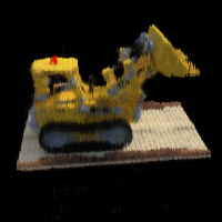
Across the training process, here are some prediction results on the test set at different steps:

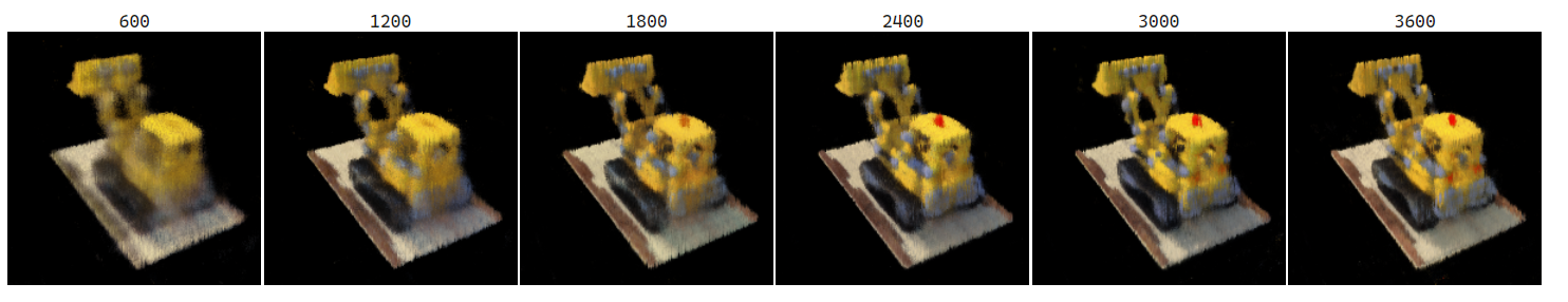
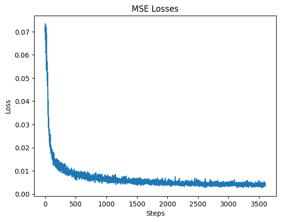
The views start off extremely blurry, and there’s visible improvement to clarity across as training progressed. At step 3600, the edges are much more distinct and more details are visible. This improvement in accuracy is also reflected in the MSE and PSNR losses, as shown in the graphs below. The PSNR does oscillate a bit as the training went on. It was able to achieve above 23 PSNR and did not exceed 26.

Final Results

Some of the novel views from the test set:

See the complete gif here:

Bells & Whistles

I choose to render depth instead of color. To do this, I replaced the color inputs to the volume rendering with the depth of the sampled points. Checkout the gif below: