Shoot Pictures

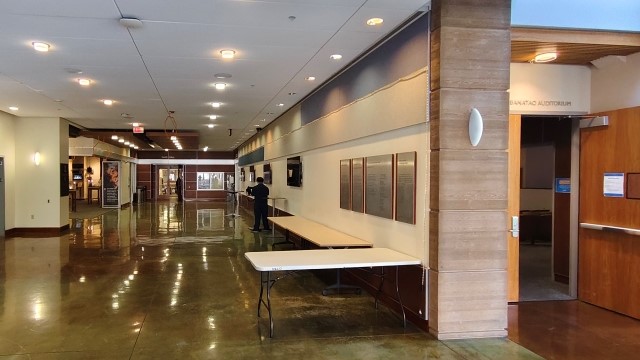
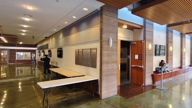
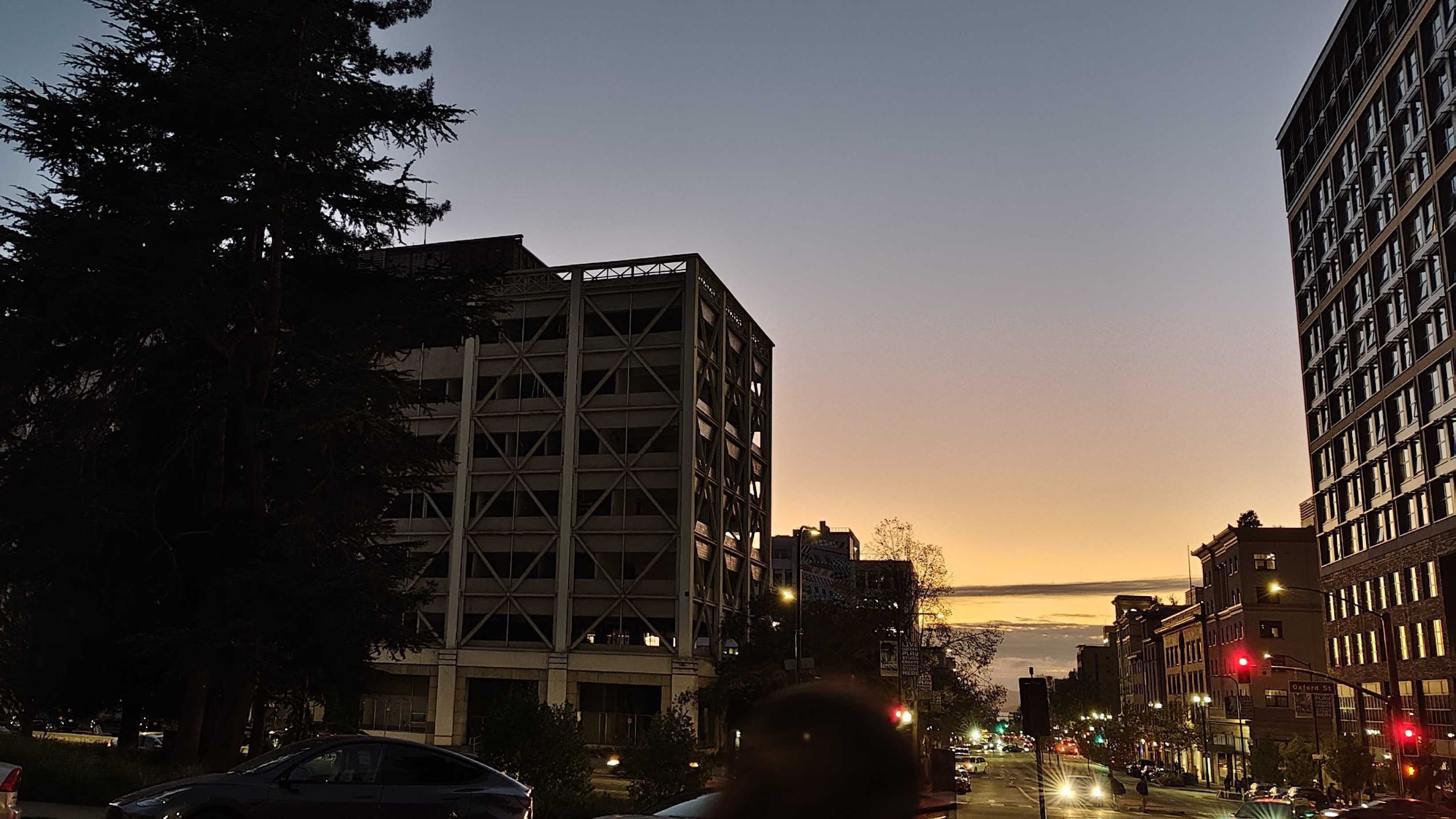
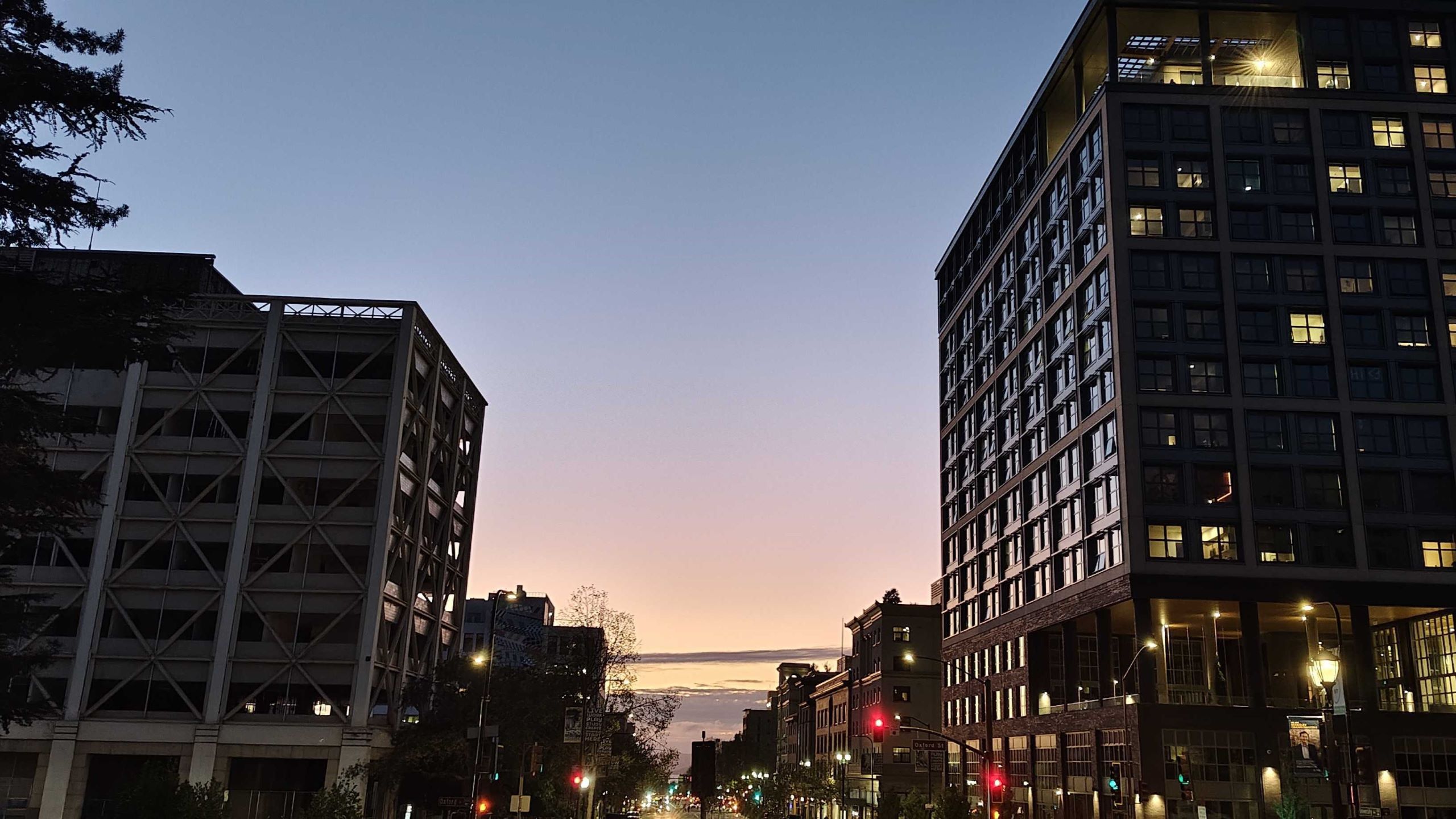
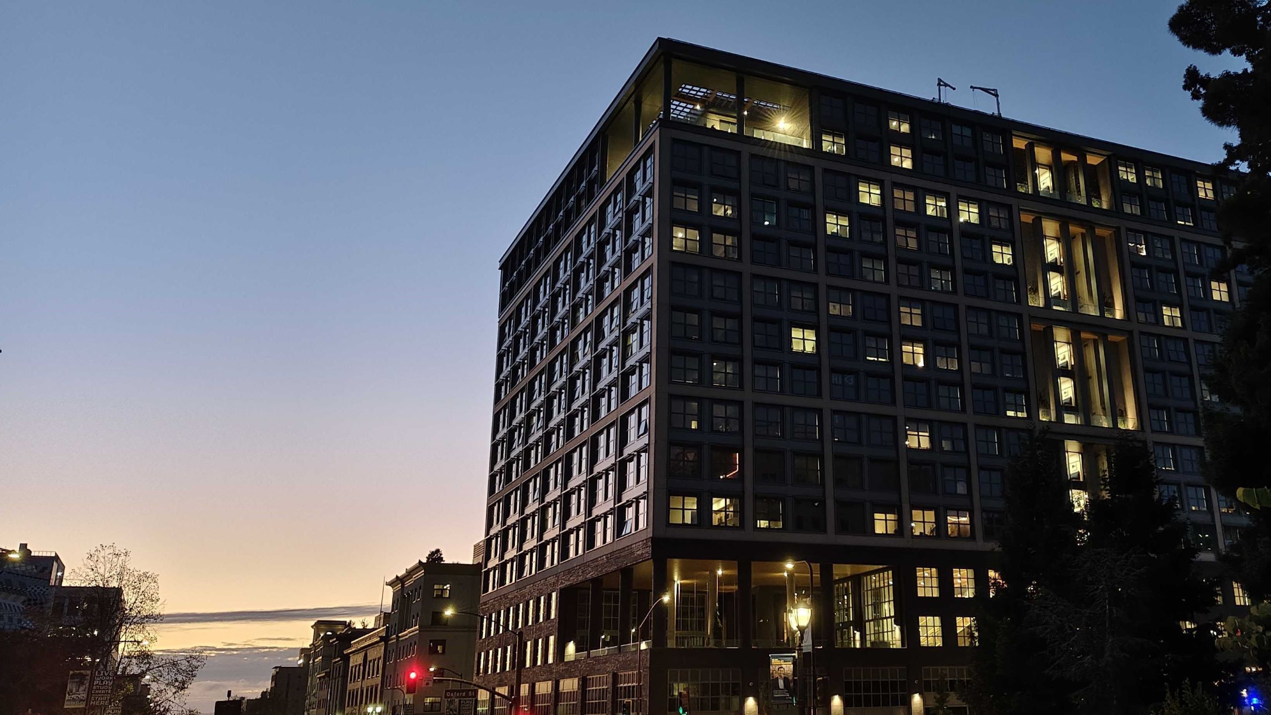
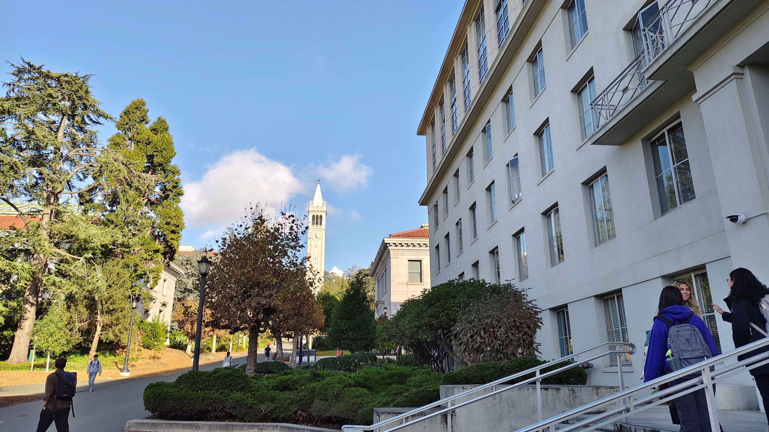
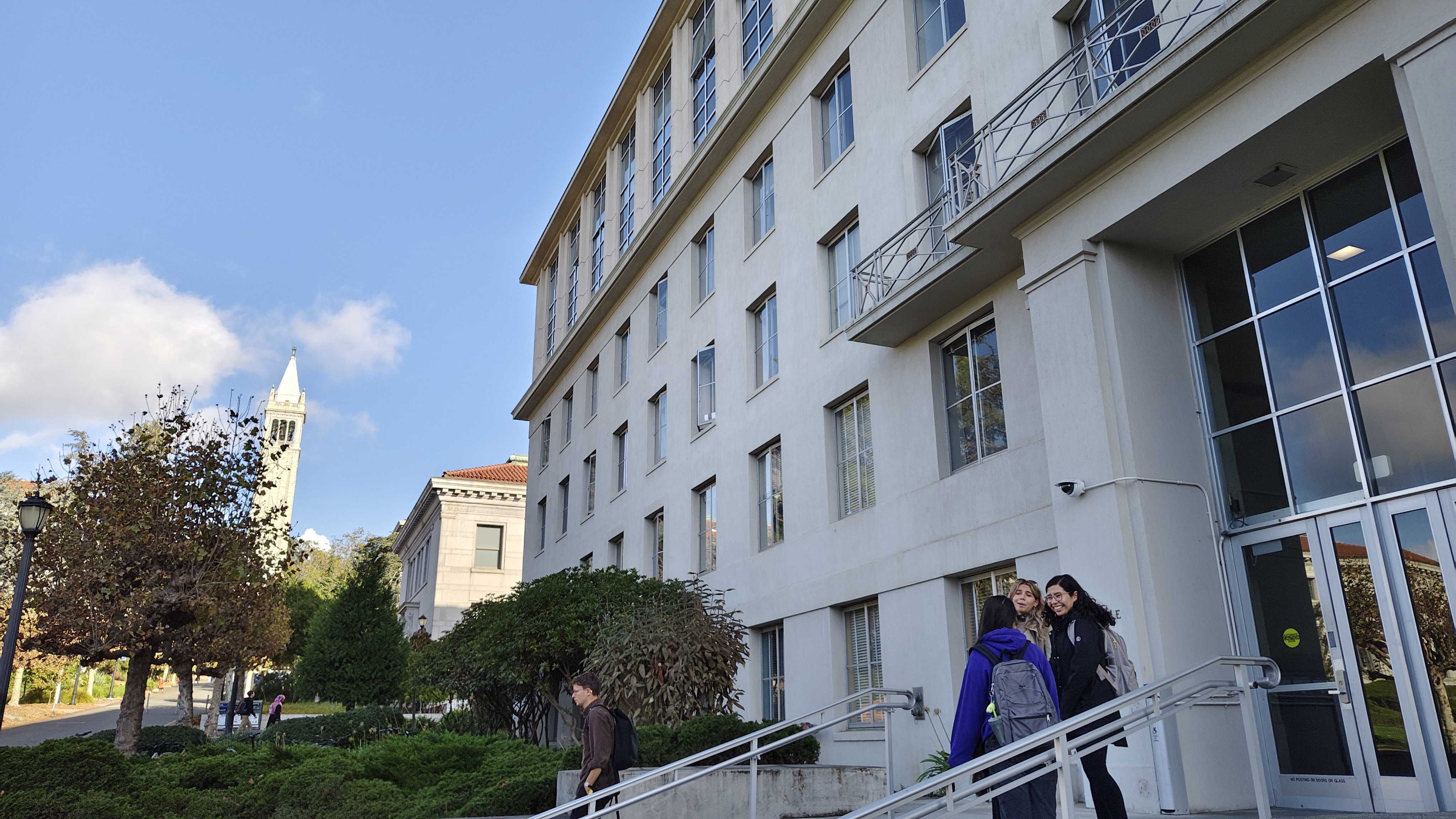
I took 2 images in the Sutardja Dai Hall at the corner of the hall way:

Recover Homography

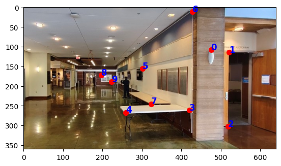
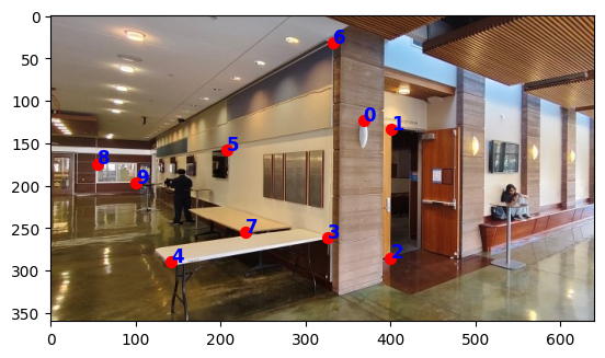
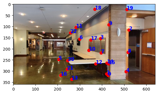
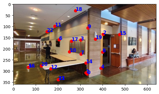
I used the point correspondence tool from project 3 and clicked 10 corresponding points on the images. I displayed the points with matplotlib:

Here’s the linear system of equations for the 8 variables in the homography:

For each point, I stacked the 2 linear equations to the left and the corresponding coordinates on the right. I used np.linalg.lstsq to find the best fitting solution to the system.

Warp Images

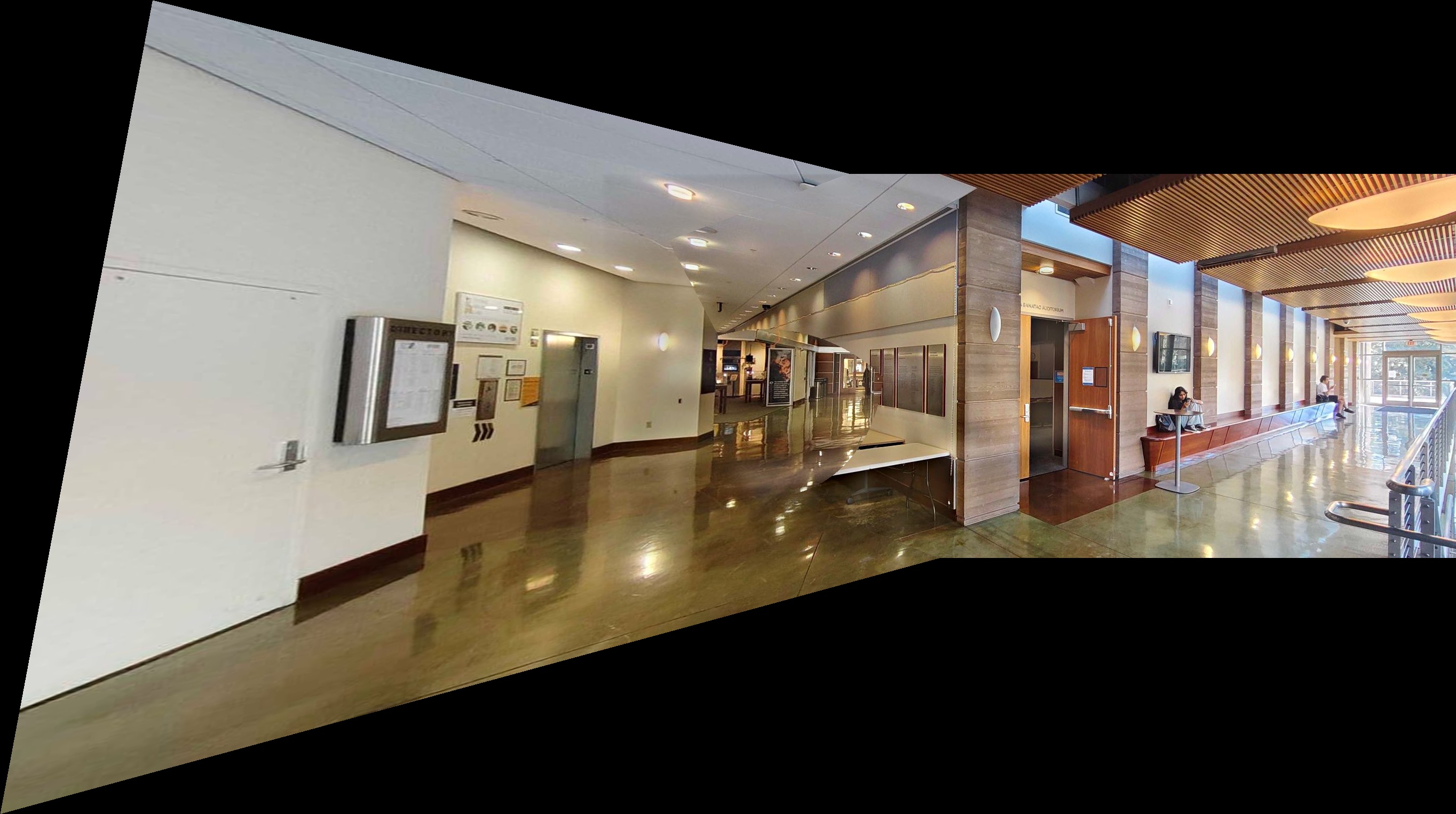
Here are the results of warping the full images:

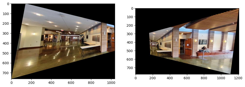
Image Rectification

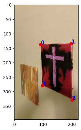
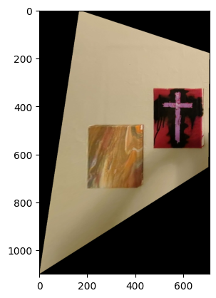
I chose to rectify another image. It’s an angled image of 2 paintings in my apartment. On the right is the recification results. Looks pretty nice!

Blend Mosaic

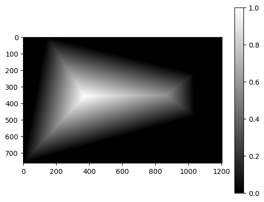
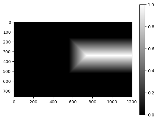
I used the distance transform alpha masking method. Here are the masks (left image warped, right kept the same):

For low frequencies, I compute a weighted average according to the distance to the edge. For high frequencies, I select the pixel where the distance transform mask has greater value. Here are the results of mosaicing the hall way in Sutardja Dai:

Harris Interest Point Detector

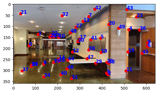
I used the starter code linked to in the project. Before passing the image to the harris corner detection function, I bias/gain-normalized the grayscale images. I also set the threshold_rel parameter of peak_local_max to 0.01 to filter some points. Results from the left interior image of Sutardja Dai:

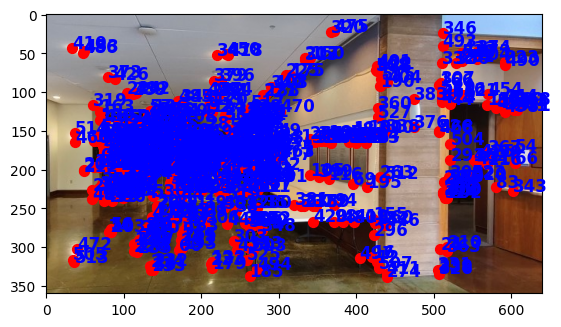
There are a lot of cluttered points. Let’s eliminate some of them in the next step.

Adaptive NMS

Overview of ANMS:

• get the pair-wise distances between all corners selected in the previous step.

• for each point, check all other points for robustness. If a closer point is found, update the current point’s radius

• return the coordinates with top k radii.

I’m picking the top 50 points after ANMS. They are much more evenly spread out across the image.

Feature Extraction

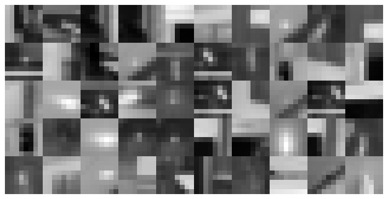
I get a 40x40 pixel block around the remaining coordinates, and downsample them to 8x8. Here are the extrations for the left image:

Feature Matching

To do feature matching, I adopt the metric of the ratio between first nearest neighbor and second nearest neighbor. Overview of the procedure:

• flatten all 8x8 feature squares

• calculate pair-wise squared euclidean distances between the features in image1 and those in image 2

• for each feature in image1, find the top 2 nearest neighbors in image 2.
  • calculate the ratio between these distances,
  • if under threshold (set to ~0.66 according to graphs in paper), declare the features a match

• return all matched points.

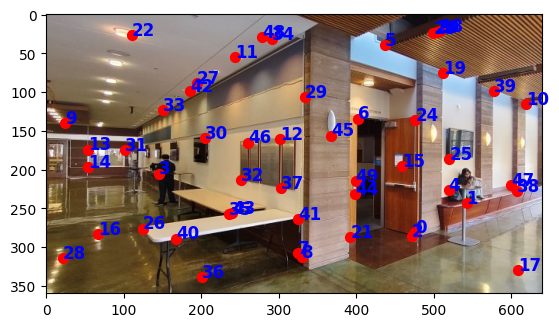
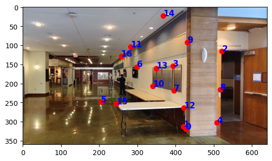
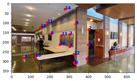
Here are the results:

RANSAC

To select inliers to match with each other and avoid outliers (for example, in the images above the point labeled 19 is an outlier) messing with the homography, I implemented RANSAC according to the description of the algorithm in lecture. I got these matches:

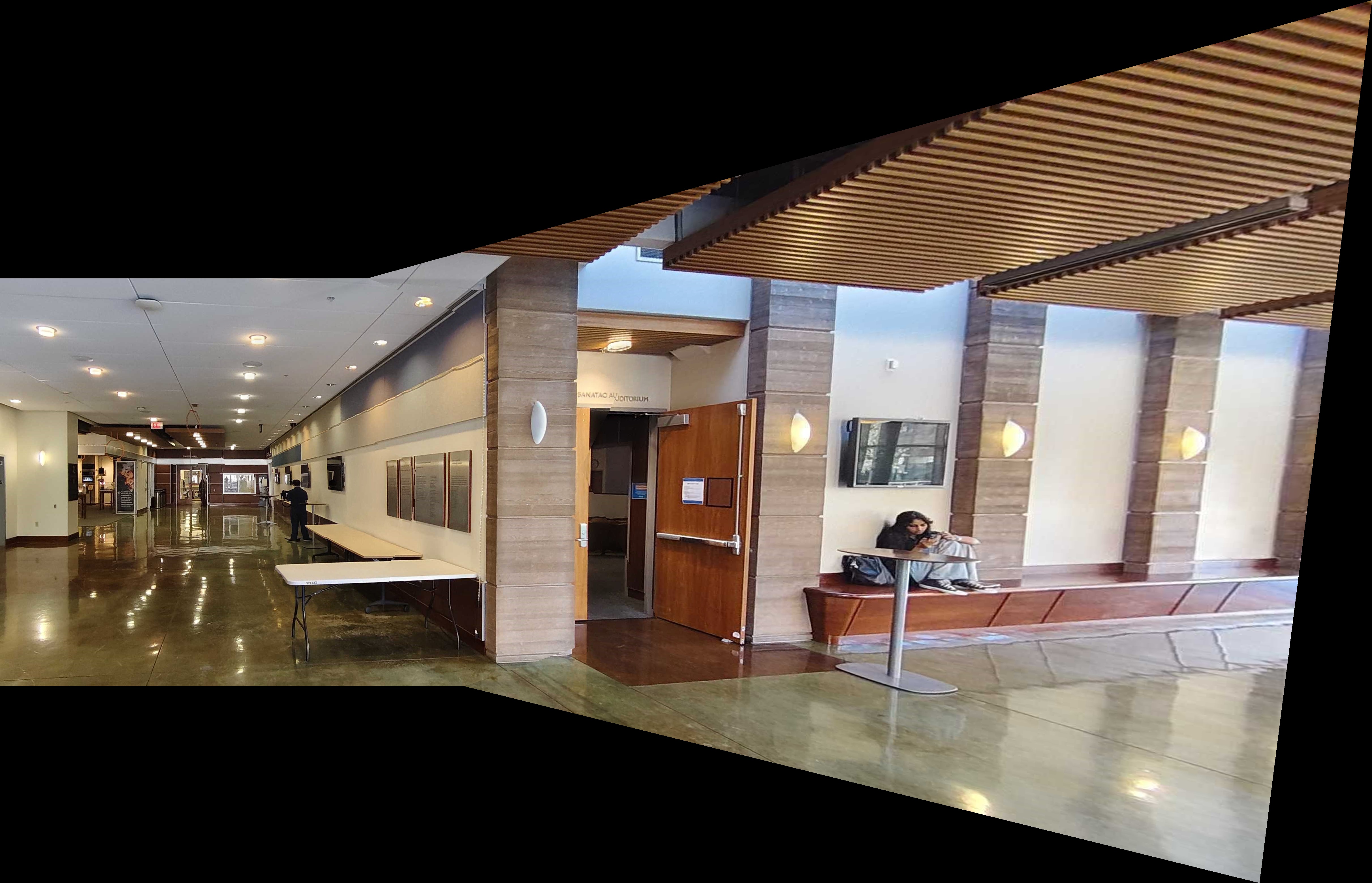
And I got the mosaic for these 2 images

compared to the manuel point matching:

Other Mosaics

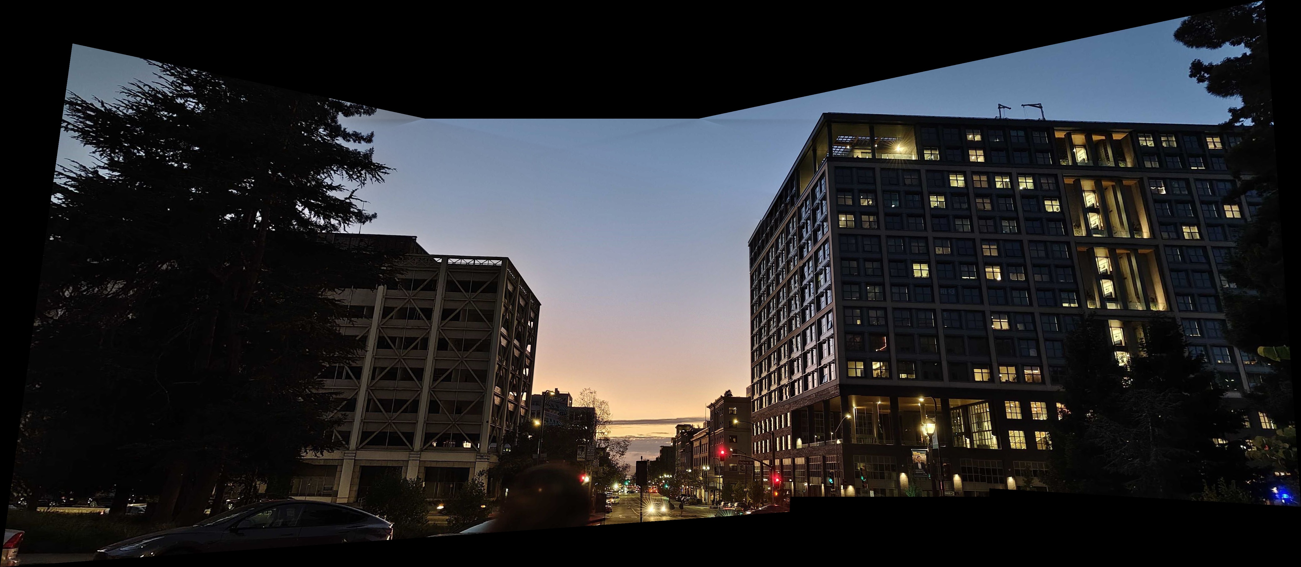
Anchor House:

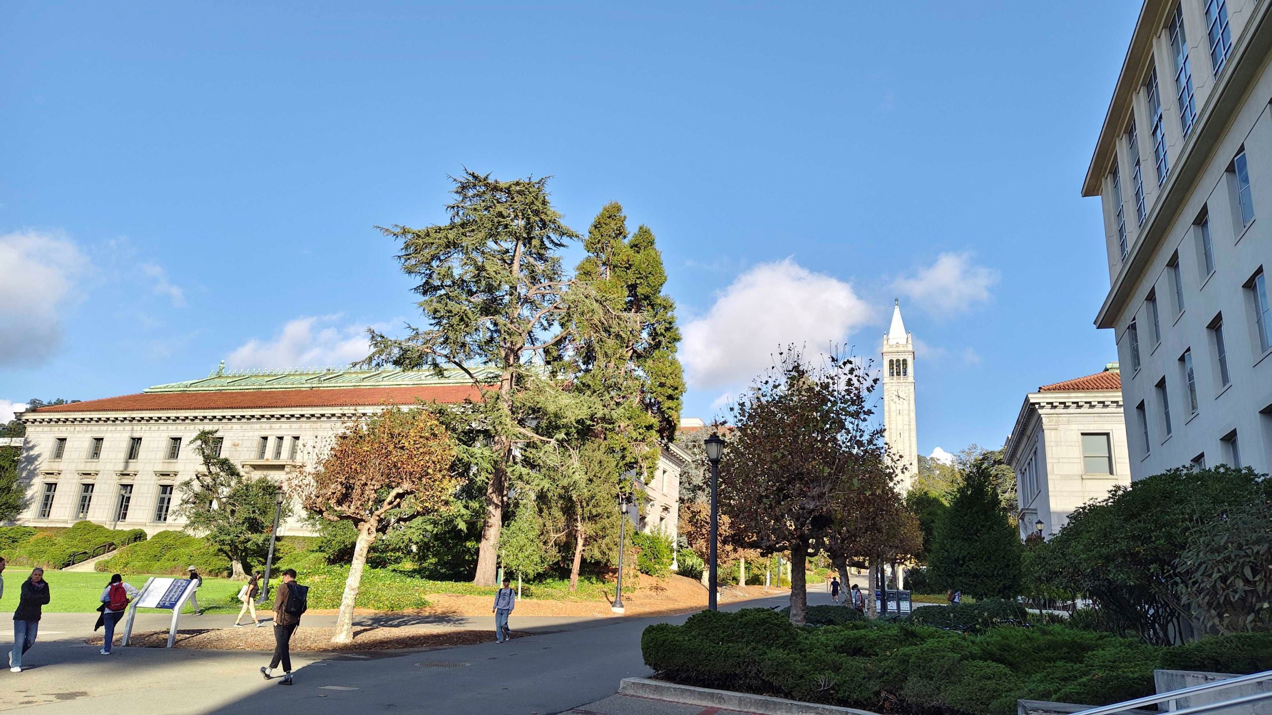
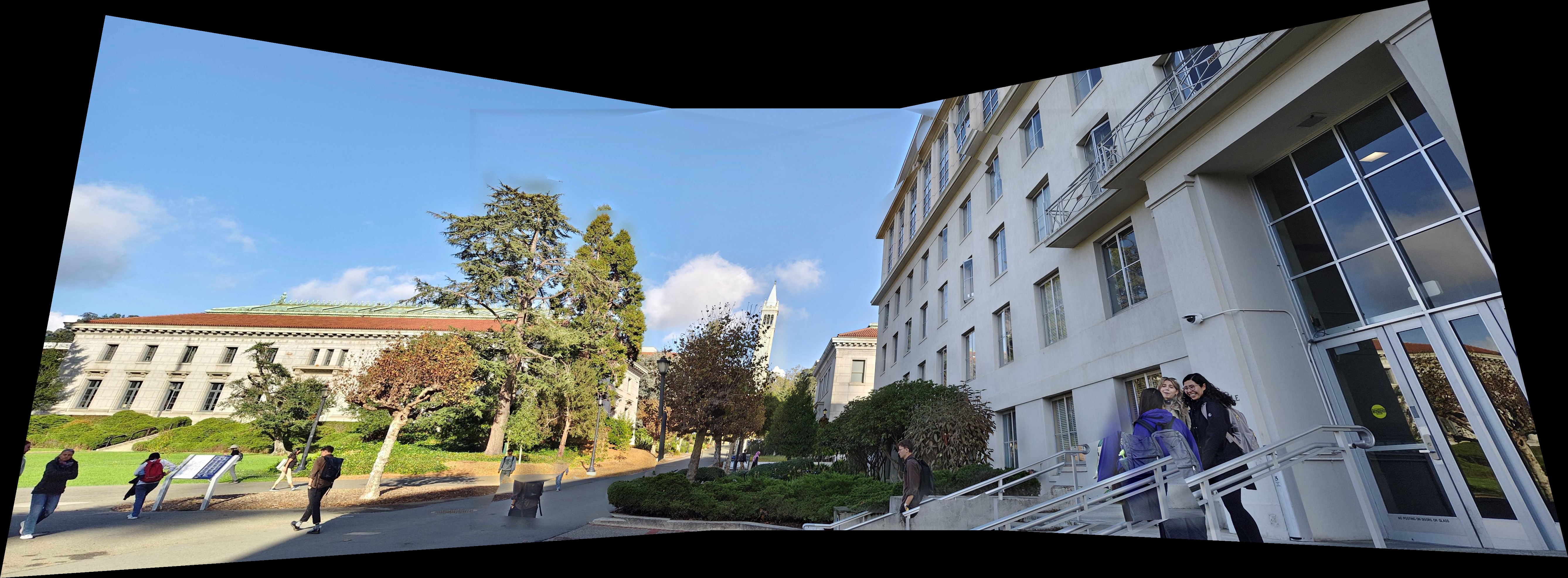
Outside Dwinelle

What I learned

• blending is still an important and difficult step. even if you have really good matching, blending is still super important

• it’s hard to set a single hyperparameter for different thresholds (for example, for e_1nn / e_2nn, for how many points to keep in AMNS, for how many iterations to do RANSAC, etc.). at lof of manuel work is still required, despite having these great matching techniques

• memory management is important. the processing times of these procedures can be long, especially for warping. and you don’t want you jupyter kernel to die on you in the middle of blending.